Using COPASI via BasiCO

This notebook demonstrates how to apply pyABC to models simulated via COPASI, using the Python interface BasiCO.

pyABC’s COPASI/BasiCO interface is the class pyabc.copasi.BasicoModel.

# install if not done yet
!pip install pyabc[copasi] --quiet

import tempfile

import matplotlib.pyplot as plt
import numpy as np

import pyabc
from pyabc.copasi import BasicoModel

pyabc.settings.set_figure_params('pyabc')  # for beautified plots

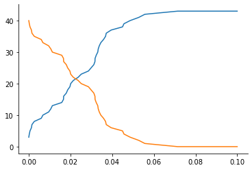
We consider a simple reaction \(m_1: X + Y \xrightarrow{k_1} 2Y\) (used already in the model selection notebook), simulated as a discrete jump process. The model is defined in an XML file in the SBML format. See the COPASI and BasiCO documentation for WYSIWYG or programmatic ways of constructing such model files. Note that other simulation methods are available, see the BasicoModel API documentation for details.

max_t = 0.1
model = BasicoModel("models/model1.xml", duration=max_t)

true_par = {"rate": 2.3}
obs = model(true_par)
plt.plot(obs["t"], obs["X"]);

As usual, we define a distance and a prior distribution.

n_test_times = 20
t_test_times = np.linspace(0, max_t, n_test_times)


def distance(x, y):
    xt_ind = np.searchsorted(x["t"], t_test_times) - 1
    yt_ind = np.searchsorted(y["t"], t_test_times) - 1
    error = (
        np.absolute(x["X"][:, 1][xt_ind] - y["X"][:, 1][yt_ind]).sum()
        / t_test_times.size
    )
    return error


prior = pyabc.Distribution(rate=pyabc.RV("uniform", 0, 50))

We are all set to run an analysis:

abc = pyabc.ABCSMC(model, prior, distance, population_size=100)
db = tempfile.mkstemp(suffix=".db")[1]
abc.new("sqlite:///" + db, obs)
h = abc.run(max_nr_populations=10, min_acceptance_rate=1e-2)

ABC.Sampler INFO: Parallelize sampling on 4 processes.
INFO:ABC.Sampler:Parallelize sampling on 4 processes.
ABC.History INFO: Start <ABCSMC id=1, start_time=2021-12-05 12:15:57>
INFO:ABC.History:Start <ABCSMC id=1, start_time=2021-12-05 12:15:57>
ABC INFO: Calibration sample t = -1.
INFO:ABC:Calibration sample t = -1.
ABC INFO: t: 0, eps: 8.95000000e+00.
INFO:ABC:t: 0, eps: 8.95000000e+00.
ABC INFO: Accepted: 100 / 208 = 4.8077e-01, ESS: 1.0000e+02.
INFO:ABC:Accepted: 100 / 208 = 4.8077e-01, ESS: 1.0000e+02.
ABC INFO: t: 1, eps: 8.25000000e+00.
INFO:ABC:t: 1, eps: 8.25000000e+00.
ABC INFO: Accepted: 100 / 206 = 4.8544e-01, ESS: 9.6966e+01.
INFO:ABC:Accepted: 100 / 206 = 4.8544e-01, ESS: 9.6966e+01.
ABC INFO: t: 2, eps: 6.55009972e+00.
INFO:ABC:t: 2, eps: 6.55009972e+00.
ABC INFO: Accepted: 100 / 250 = 4.0000e-01, ESS: 9.5430e+01.
INFO:ABC:Accepted: 100 / 250 = 4.0000e-01, ESS: 9.5430e+01.
ABC INFO: t: 3, eps: 5.09217796e+00.
INFO:ABC:t: 3, eps: 5.09217796e+00.
ABC INFO: Accepted: 100 / 226 = 4.4248e-01, ESS: 9.8080e+01.
INFO:ABC:Accepted: 100 / 226 = 4.4248e-01, ESS: 9.8080e+01.
ABC INFO: t: 4, eps: 3.08808133e+00.
INFO:ABC:t: 4, eps: 3.08808133e+00.
ABC INFO: Accepted: 100 / 307 = 3.2573e-01, ESS: 9.6889e+01.
INFO:ABC:Accepted: 100 / 307 = 3.2573e-01, ESS: 9.6889e+01.
ABC INFO: t: 5, eps: 1.92108500e+00.
INFO:ABC:t: 5, eps: 1.92108500e+00.
ABC INFO: Accepted: 100 / 355 = 2.8169e-01, ESS: 9.2695e+01.
INFO:ABC:Accepted: 100 / 355 = 2.8169e-01, ESS: 9.2695e+01.
ABC INFO: t: 6, eps: 1.47554023e+00.
INFO:ABC:t: 6, eps: 1.47554023e+00.
ABC INFO: Accepted: 100 / 489 = 2.0450e-01, ESS: 5.8759e+01.
INFO:ABC:Accepted: 100 / 489 = 2.0450e-01, ESS: 5.8759e+01.
ABC INFO: t: 7, eps: 1.20000000e+00.
INFO:ABC:t: 7, eps: 1.20000000e+00.
ABC INFO: Accepted: 100 / 1043 = 9.5877e-02, ESS: 8.4161e+01.
INFO:ABC:Accepted: 100 / 1043 = 9.5877e-02, ESS: 8.4161e+01.
ABC INFO: t: 8, eps: 1.05000000e+00.
INFO:ABC:t: 8, eps: 1.05000000e+00.
ABC INFO: Accepted: 100 / 1556 = 6.4267e-02, ESS: 8.3430e+01.
INFO:ABC:Accepted: 100 / 1556 = 6.4267e-02, ESS: 8.3430e+01.
ABC INFO: t: 9, eps: 9.50000000e-01.
INFO:ABC:t: 9, eps: 9.50000000e-01.
ABC INFO: Accepted: 100 / 2819 = 3.5474e-02, ESS: 9.1430e+01.
INFO:ABC:Accepted: 100 / 2819 = 3.5474e-02, ESS: 9.1430e+01.
ABC INFO: Stop: Maximum number of generations.
INFO:ABC:Stop: Maximum number of generations.
ABC.History INFO: Done <ABCSMC id=1, duration=0:00:16.694937, end_time=2021-12-05 12:16:14>
INFO:ABC.History:Done <ABCSMC id=1, duration=0:00:16.694937, end_time=2021-12-05 12:16:14>

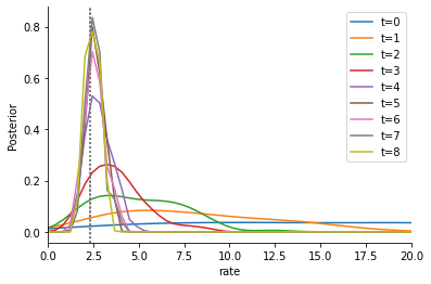
As usual, we can now analyze the results. Posterior approximation over time:

fig, ax = plt.subplots()

for t in range(h.max_t):
    pyabc.visualization.plot_kde_1d_highlevel(
        h,
        x="rate",
        xmin=0,
        xmax=20,
        t=t,
        refval=true_par,
        refval_color="grey",
        label=f"t={t}",
        ax=ax,
    )
ax.legend();

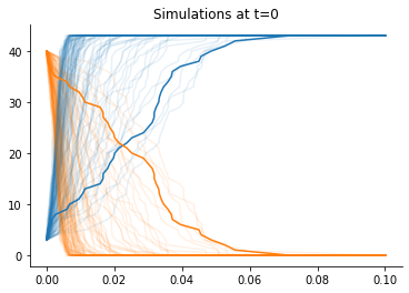
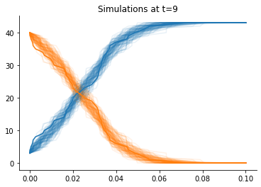
Accepted simulations at the beginning and at the end:

def plot_data(sumstat, weight, ax, **kwargs):
    """Plot a single trajectory"""
    for i in range(2):
        ax.plot(sumstat["t"], sumstat['X'][:, i], color=f"C{i}", alpha=0.1)


for t in [0, h.max_t]:
    _, ax = plt.subplots()
    pyabc.visualization.plot_data_callback(
        h,
        plot_data,
        t=t,
        ax=ax,
    )
    ax.plot(obs["t"], obs["X"])
    ax.set_title(f"Simulations at t={t}");