Model selection

Here is a small example on how to do Bayesian model selection.

There are more examples in the examples section of the documentation, such as a parameter inference example with a single model only.

The notebook can be downloaded here: Model selection.

The following classes from the pyABC package are used for this example:

• ABCSMC

• RV

• Distribution

• PercentileDistance

# install if not done yet
!pip install pyabc --quiet

Defining the model

To do model selection, we first need some models. A model, in the simplest case, is just a callable which takes a single dict as input and returns a single dict as output. The keys of the input dictionary are the parameters of the model, the output keys denote the summary statistics. Here, the dict is passed as parameters and has the entry x, which denotes the mean of a Gaussian. It returns the observed summary statistics y, which is just the sampled value.

%matplotlib inline
import os
import tempfile

import scipy.stats as st

import pyabc

pyabc.settings.set_figure_params('pyabc')  # for beautified plots

# Define a gaussian model

sigma = 0.5


def model(parameters):
    # sample from a gaussian
    y = st.norm(parameters.x, sigma).rvs()
    # return the sample as dictionary
    return {"y": y}

For model selection we usually have more than one model. These are assembled in a list. We require a Bayesian prior over the models. The default is to have a uniform prior over the model classes. This concludes the model definition.

# We define two models, but they are identical so far
models = [model, model]

# However, our models' priors are not the same.
# Their mean differs.
mu_x_1, mu_x_2 = 0, 1
parameter_priors = [
    pyabc.Distribution(x=pyabc.RV("norm", mu_x_1, sigma)),
    pyabc.Distribution(x=pyabc.RV("norm", mu_x_2, sigma)),
]

Configuring the ABCSMC run

Having the models defined, we can plug together the ABCSMC class. We need a distance function, to measure the distance of obtained samples.

# We plug all the ABC options together
abc = pyabc.ABCSMC(
    models, parameter_priors, pyabc.PercentileDistance(measures_to_use=["y"])
)

INFO:Sampler:Parallelizing the sampling on 4 cores.

Setting the observed data

Actually measured data can now be passed to the ABCSMC. This is set via the new method, indicating that we start a new run as opposed to resuming a stored run (see the “resume stored run” example). Moreover, we have to set the output database where the ABC-SMC run is logged.

# y_observed is the important piece here: our actual observation.
y_observed = 1
# and we define where to store the results
db_path = "sqlite:///" + os.path.join(tempfile.gettempdir(), "test.db")
history = abc.new(db_path, {"y": y_observed})

INFO:History:Start <ABCSMC id=1, start_time=2021-02-21 20:27:46.032578>

The new method returns a history object, whose id identifies the ABC-SMC run in the database. We’re not using this id for now. But it might be important when you load the stored data or want to continue an ABC-SMC run in the case of having more than one ABC-SMC run stored in a single database.

print("ABC-SMC run ID:", history.id)

ABC-SMC run ID: 1

Running the ABC

We run the ABCSMC specifying the epsilon value at which to terminate. The default epsilon strategy is the pyabc.epsilon.MedianEpsilon. Whatever is reached first, the epsilon or the maximum number allowed populations, terminates the ABC run. The method returns a pyabc.storage.History object, which can, for example, be queried for the posterior probabilities.

# We run the ABC until either criterion is met
history = abc.run(minimum_epsilon=0.2, max_nr_populations=5)

INFO:ABC:Calibration sample t=-1.
INFO:Epsilon:initial epsilon is 0.4513005593964347
INFO:ABC:t: 0, eps: 0.4513005593964347.
INFO:ABC:Acceptance rate: 100 / 221 = 4.5249e-01, ESS=1.0000e+02.
INFO:ABC:t: 1, eps: 0.18718437297658125.
INFO:ABC:Acceptance rate: 100 / 353 = 2.8329e-01, ESS=8.8666e+01.
INFO:pyabc.util:Stopping: minimum epsilon.
INFO:History:Done <ABCSMC id=1, duration=0:00:02.979904, end_time=2021-02-21 20:27:49.012482>

Note that the history object is also always accessible from the ABCSMC object:

history is abc.history

True

Visualization and analysis of results

The pyabc.storage.History> object can, for example, be queried for the posterior probabilities in the populations:

# Evaluate the model probabililties
model_probabilities = history.get_model_probabilities()
model_probabilities

m	0	1
t
0	0.33000	0.67000
1	0.25232	0.74768

And now, let’s visualize the results:

pyabc.visualization.plot_model_probabilities(history)

<AxesSubplot:title={'center':'Model probabilities'}, xlabel='Population index', ylabel='Probability'>

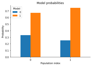
So model 1 is the more probable one. Which is expected as it was centered at 1 and the observed data was also 1, whereas model 0 was centered at 0, which is farther away from the observed data.