Using Julia via pyjulia

This notebook demonstrates the application of pyABC to models defined in Julia.

pyABC’s Julia interface is the class pyabc.external.julia.Julia.

import tempfile

import matplotlib.pyplot as plt

import pyabc
from pyabc import ABCSMC, RV, Distribution, MulticoreEvalParallelSampler
from pyabc.external.julia import Julia

pyabc.settings.set_figure_params('pyabc')  # for beautified plots

As demonstration example, we use an SIR disease dynamics model. For simulation, we use an implementation of Gillespie’s direct algorithm in the DifferentialEquations.jl package.

The code consists of multiple functions in the file model_julia/SIR.jl, wrapped in the namespace of a module SIR. Importing the module and dependencies can take some time due to pre-processing.

%%time
jl = Julia(module_name="SIR", source_file="model_julia/SIR.jl")

CPU times: user 33.7 s, sys: 1.46 s, total: 35.1 s
Wall time: 34.9 s

jl.display_source_ipython()

module SIR

# Install dependencies
using Pkg
Pkg.add("Catalyst")
Pkg.add("DiffEqJump")

# Define reaction network
using Catalyst
sir_model = @reaction_network begin
    r1, S + I --> 2I
    r2, I --> R
end r1 r2

# ground truth parameter
p = (0.0001, 0.01)
# initial state
u0 = [999, 1, 0]
# time span
tspan = (0.0, 250.0)
# formulate as discrete problem
prob  = DiscreteProblem(sir_model, u0, tspan, p)

# formulate as Markov jump process
using DiffEqJump
jump_prob = JumpProblem(
    sir_model, prob, Direct(), save_positions=(false, false),
)

"""
Simulate model for parameters `10.0.^par`.
"""
function model(par)
    p = 10.0.^((par["p1"], par["p2"]))
    sol = solve(remake(jump_prob, p=p), SSAStepper(), saveat=2.5)
    return Dict("t"=>sol.t, "u"=>sol.u)
end

# observed data
observation = model(Dict("p1"=>log10(p[1]), "p2"=>log10(p[2])))

"""
Distance between model simulations or observed data `y` and `y0`.
"""
function distance(y, y0)
    u, u0 = y["u"], y0["u"]
    if length(u) != length(u0)
        throw(AssertionError("Dimension mismatch"))
    end
    return sum((u .- u0).^2) / length(u0)
end

end  # module

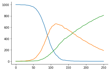
The Julia code defines functions for model and distance. The model returns a dictionary, whose entries are internally converted to numpy arrays, while the distance returns a single floating value. Further, also the observed data can be defined in and imported from Julia. Note that also only a subset of model, distance and observation can be defined in Julia, and combined with Python objects.

model = jl.model()
distance = jl.distance()
obs = jl.observation()

_ = plt.plot(obs["t"], obs["u"])

We use a prior on log-scale, the Julia model applies the corresponding transformation internally.

gt_par = {"p1": -4.0, "p2": -2.0}

# parameter limits and prior
par_limits = {
    "p1": (-5, -3),
    "p2": (-3, -1),
}
prior = Distribution(
    **{key: RV("uniform", lb, ub - lb) for key, (lb, ub) in par_limits.items()}
)

If we use parallelization, we need to call all julia functions once before, to perform necessary pre-compiling:

distance(model(gt_par), model(gt_par))

297286.7590759076

We are all set to run an analysis, even with parallelization via multi-processing:

abc = ABCSMC(
    model,
    prior,
    distance,
    sampler=MulticoreEvalParallelSampler(),
)
db = tempfile.mkstemp(suffix=".db")[1]
abc.new("sqlite:///" + db, obs)
h = abc.run(max_nr_populations=10)

ABC.Sampler INFO: Parallelize sampling on 4 processes.
ABC.History INFO: Start <ABCSMC id=1, start_time=2021-11-18 17:21:06>
ABC INFO: Calibration sample t = -1.
ABC INFO: t: 0, eps: 2.18842571e+05.
ABC INFO: Accepted: 100 / 212 = 4.7170e-01, ESS: 1.0000e+02.
ABC INFO: t: 1, eps: 1.45222795e+05.
ABC INFO: Accepted: 100 / 203 = 4.9261e-01, ESS: 7.8092e+01.
ABC INFO: t: 2, eps: 8.71552898e+04.
ABC INFO: Accepted: 100 / 268 = 3.7313e-01, ESS: 8.9681e+01.
ABC INFO: t: 3, eps: 5.17737477e+04.
ABC INFO: Accepted: 100 / 211 = 4.7393e-01, ESS: 9.0513e+01.
ABC INFO: t: 4, eps: 2.39628036e+04.
ABC INFO: Accepted: 100 / 346 = 2.8902e-01, ESS: 9.3795e+01.
ABC INFO: t: 5, eps: 1.14595719e+04.
ABC INFO: Accepted: 100 / 317 = 3.1546e-01, ESS: 8.1326e+01.
ABC INFO: t: 6, eps: 6.61310965e+03.
ABC INFO: Accepted: 100 / 403 = 2.4814e-01, ESS: 8.4728e+01.
ABC INFO: t: 7, eps: 3.66662784e+03.
ABC INFO: Accepted: 100 / 556 = 1.7986e-01, ESS: 6.2655e+01.
ABC INFO: t: 8, eps: 1.90359721e+03.
ABC INFO: Accepted: 100 / 683 = 1.4641e-01, ESS: 9.1709e+01.
ABC INFO: t: 9, eps: 1.02475108e+03.
ABC INFO: Accepted: 100 / 989 = 1.0111e-01, ESS: 7.6864e+01.
ABC INFO: Stop: Maximum number of generations.
ABC.History INFO: Done <ABCSMC id=1, duration=0:00:12.231150, end_time=2021-11-18 17:21:19>

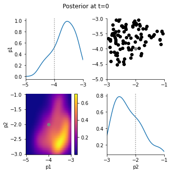
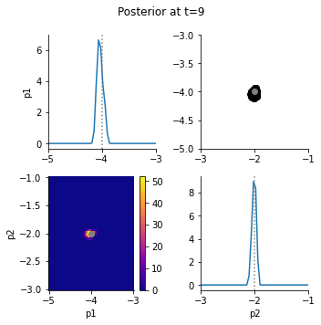
The posterior marginals show that the data constrain the parameters well:

for t in [0, h.max_t]:
    pyabc.visualization.plot_kde_matrix_highlevel(
        h,
        t=t,
        limits=par_limits,
        refval=gt_par,
        refval_color="grey",
    )
    plt.gcf().suptitle(f"Posterior at t={t}")
    plt.gcf().tight_layout();

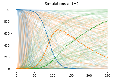
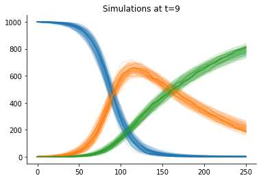
The accepted simulations closely match the observed data well, as we can see from data plots:

def plot_data(sumstat, weight, ax, **kwargs):
    """Plot a single trajectory"""
    for i in range(3):
        ax.plot(sumstat["t"], sumstat['u'][:, i], color=f"C{i}", alpha=0.1)


for t in [0, h.max_t]:
    _, ax = plt.subplots()
    pyabc.visualization.plot_data_callback(
        h,
        plot_data,
        t=t,
        ax=ax,
    )
    ax.plot(obs["t"], obs["u"])
    ax.set_title(f"Simulations at t={t}");