Aggregating and weighting diverse data
In this notebook, we illustrate the aggregation of various data, and how to combine that with an adaptive scheme of computing weights.
Aggregating diverse distance functions
We want to combine different distance metrics operating on subsets of the data to one distance value. As a toy model, assume we want to combine a Laplace and a Normal distance.
[ ]:
# install if not done yet
!pip install pyabc --quiet
[1]:
import os
import tempfile

import matplotlib.pyplot as plt
import numpy as np

import pyabc

p_true = {'p0': 0, 'p1': 0}


def model(p):
    return {
        's0': p['p0'] + 0.1 * np.random.normal(),
        's1': p['p1'] + 0.1 * np.random.normal(),
    }


observation = {'s0': 0, 's1': 0}


def distance0(x, x_0):
    return abs(x['s0'] - x_0['s0'])


def distance1(x, x_0):
    return (x['s1'] - x_0['s1']) ** 2


# prior
prior = pyabc.Distribution(
    p0=pyabc.RV('uniform', -1, 2), p1=pyabc.RV('uniform', -1, 2)
)
The key is now to use pyabc.distance.AggregatedDistance to combine both.
[2]:
distance = pyabc.AggregatedDistance([distance0, distance1])

abc = pyabc.ABCSMC(model, prior, distance)
db_path = 'sqlite:///' + os.path.join(tempfile.gettempdir(), 'tmp.db')
abc.new(db_path, observation)
history1 = abc.run(max_nr_populations=6)

# plotting


def plot_history(history):
    fig, ax = plt.subplots()
    for t in range(history.max_t + 1):
        df, w = history.get_distribution(m=0, t=t)
        pyabc.visualization.plot_kde_1d(
            df,
            w,
            xmin=-1,
            xmax=1,
            x='p0',
            ax=ax,
            label=f'PDF t={t}',
            refval=p_true,
        )
    ax.legend()

    fig, ax = plt.subplots()
    for t in range(history.max_t + 1):
        df, w = history.get_distribution(m=0, t=t)
        pyabc.visualization.plot_kde_1d(
            df,
            w,
            xmin=-1,
            xmax=1,
            x='p1',
            ax=ax,
            label=f'PDF t={t}',
            refval=p_true,
        )
    ax.legend()


plot_history(history1)
ABC.Sampler INFO: Parallelize sampling on 4 processes.
ABC.History INFO: Start <ABCSMC id=1, start_time=2021-05-19 15:19:12>
ABC INFO: Calibration sample t = -1.
ABC INFO: t: 0, eps: 7.93828347e-01.
ABC INFO: Accepted: 100 / 227 = 4.4053e-01, ESS: 1.0000e+02.
ABC INFO: t: 1, eps: 5.47513600e-01.
ABC INFO: Accepted: 100 / 227 = 4.4053e-01, ESS: 9.3165e+01.
ABC INFO: t: 2, eps: 3.48865157e-01.
ABC INFO: Accepted: 100 / 192 = 5.2083e-01, ESS: 8.7158e+01.
ABC INFO: t: 3, eps: 2.17783825e-01.
ABC INFO: Accepted: 100 / 249 = 4.0161e-01, ESS: 8.8381e+01.
ABC INFO: t: 4, eps: 1.47444558e-01.
ABC INFO: Accepted: 100 / 340 = 2.9412e-01, ESS: 9.2480e+01.
ABC INFO: t: 5, eps: 8.91141994e-02.
ABC INFO: Accepted: 100 / 394 = 2.5381e-01, ESS: 7.4999e+01.
ABC INFO: Stop: Maximum number of generations.
ABC.History INFO: Done <ABCSMC id=1, duration=0:00:03.119590, end_time=2021-05-19 15:19:15>
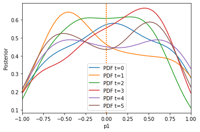
Weighted aggregation
A problem with the previous aggregation of distance function is that usually they vary on different scales. In order to account for all in a similar manner, one thing one can do is to weight them.
Let us look at a simple example of two summary statistics which vary on very different scales:
[3]:
import os
import tempfile

import pyabc

p_true = {'p0': 0, 'p1': 0}


def model(p):
    return {
        's0': p['p0'] + 0.1 * np.random.normal(),
        's1': p['p1'] + 100 * np.random.normal(),
    }


observation = {'s0': 0, 's1': 0}


def distance0(x, x_0):
    return abs(x['s0'] - x_0['s0'])


def distance1(x, x_0):
    return (x['s1'] - x_0['s1']) ** 2


# prior
prior = pyabc.Distribution(
    p0=pyabc.RV('uniform', -1, 2), p1=pyabc.RV('uniform', -1, 2)
)

distance = pyabc.AggregatedDistance([distance0, distance1])

abc = pyabc.ABCSMC(model, prior, distance)
db_path = 'sqlite:///' + os.path.join(tempfile.gettempdir(), 'tmp.db')
abc.new(db_path, observation)
history1 = abc.run(max_nr_populations=6)

# plotting


def plot_history(history):
    fig, ax = plt.subplots()
    for t in range(history.max_t + 1):
        df, w = history.get_distribution(m=0, t=t)
        pyabc.visualization.plot_kde_1d(
            df,
            w,
            xmin=-1,
            xmax=1,
            x='p0',
            ax=ax,
            label=f'PDF t={t}',
            refval=p_true,
        )
    ax.legend()

    fig, ax = plt.subplots()
    for t in range(history.max_t + 1):
        df, w = history.get_distribution(m=0, t=t)
        pyabc.visualization.plot_kde_1d(
            df,
            w,
            xmin=-1,
            xmax=1,
            x='p1',
            ax=ax,
            label=f'PDF t={t}',
            refval=p_true,
        )
    ax.legend()


plot_history(history1)
ABC.Sampler INFO: Parallelize sampling on 4 processes.
ABC.History INFO: Start <ABCSMC id=2, start_time=2021-05-19 15:19:32>
ABC INFO: Calibration sample t = -1.
ABC INFO: t: 0, eps: 4.59935137e+03.
ABC INFO: Accepted: 100 / 215 = 4.6512e-01, ESS: 1.0000e+02.
ABC INFO: t: 1, eps: 1.09029894e+03.
ABC INFO: Accepted: 100 / 421 = 2.3753e-01, ESS: 9.3548e+01.
ABC INFO: t: 2, eps: 2.14142711e+02.
ABC INFO: Accepted: 100 / 784 = 1.2755e-01, ESS: 9.1347e+01.
ABC INFO: t: 3, eps: 4.48406680e+01.
ABC INFO: Accepted: 100 / 1955 = 5.1151e-02, ESS: 7.7921e+01.
ABC INFO: t: 4, eps: 1.34184695e+01.
ABC INFO: Accepted: 100 / 3585 = 2.7894e-02, ESS: 7.8617e+01.
ABC INFO: t: 5, eps: 4.69471462e+00.
ABC INFO: Accepted: 100 / 6668 = 1.4997e-02, ESS: 9.5092e+01.
ABC INFO: Stop: Maximum number of generations.
ABC.History INFO: Done <ABCSMC id=2, duration=0:00:10.112188, end_time=2021-05-19 15:19:42>
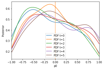
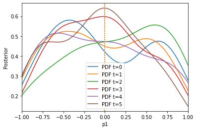
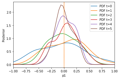
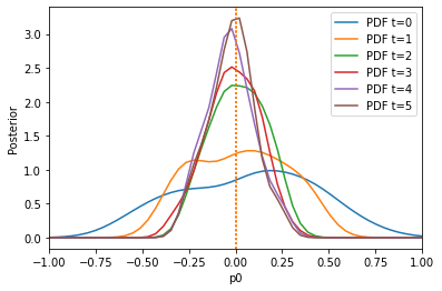
The algorithm has problems extracting information from the first summary statistic on the first parameter, because the second summary statistic is on a much larger scale. Let us use the pyabc.distance.AdaptiveAggregatedDistance instead, which tries to find good weights itself (and even adapts these weights over time):
[4]:
# prior
prior = pyabc.Distribution(
    p0=pyabc.RV('uniform', -1, 2), p1=pyabc.RV('uniform', -1, 2)
)

distance = pyabc.AdaptiveAggregatedDistance([distance0, distance1])

abc = pyabc.ABCSMC(model, prior, distance)
db_path = 'sqlite:///' + os.path.join(tempfile.gettempdir(), 'tmp.db')
abc.new(db_path, observation)
history2 = abc.run(max_nr_populations=6)

plot_history(history2)
ABC.Sampler INFO: Parallelize sampling on 4 processes.
ABC.History INFO: Start <ABCSMC id=3, start_time=2021-05-19 15:19:54>
ABC INFO: Calibration sample t = -1.
ABC.Population INFO: Recording also rejected particles: True
ABC INFO: t: 0, eps: 5.56804028e-01.
ABC INFO: Accepted: 100 / 215 = 4.6512e-01, ESS: 1.0000e+02.
ABC INFO: t: 1, eps: 3.16722119e-01.
ABC INFO: Accepted: 100 / 190 = 5.2632e-01, ESS: 9.2354e+01.
ABC INFO: t: 2, eps: 2.20958442e-01.
ABC INFO: Accepted: 100 / 346 = 2.8902e-01, ESS: 9.6911e+01.
ABC INFO: t: 3, eps: 1.61422674e-01.
ABC INFO: Accepted: 100 / 408 = 2.4510e-01, ESS: 8.1748e+01.
ABC INFO: t: 4, eps: 1.16683118e-01.
ABC INFO: Accepted: 100 / 587 = 1.7036e-01, ESS: 7.4133e+01.
ABC INFO: t: 5, eps: 6.81859941e-02.
ABC INFO: Accepted: 100 / 1256 = 7.9618e-02, ESS: 8.0627e+01.
ABC INFO: Stop: Maximum number of generations.
ABC.History INFO: Done <ABCSMC id=3, duration=0:00:04.460621, end_time=2021-05-19 15:19:59>
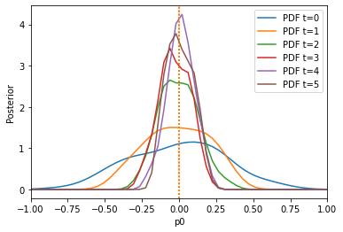
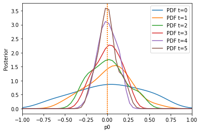
The result is much better. We can also only initially calculate weights by setting adaptive=False:
[5]:
# prior
prior = pyabc.Distribution(
    p0=pyabc.RV('uniform', -1, 2), p1=pyabc.RV('uniform', -1, 2)
)

distance = pyabc.AdaptiveAggregatedDistance(
    [distance0, distance1], adaptive=False
)

abc = pyabc.ABCSMC(model, prior, distance)
db_path = 'sqlite:///' + os.path.join(tempfile.gettempdir(), 'tmp.db')
abc.new(db_path, observation)
history3 = abc.run(max_nr_populations=6)

plot_history(history3)
ABC.Sampler INFO: Parallelize sampling on 4 processes.
ABC.History INFO: Start <ABCSMC id=4, start_time=2021-05-19 15:20:40>
ABC INFO: Calibration sample t = -1.
ABC INFO: t: 0, eps: 5.66625277e-01.
ABC INFO: Accepted: 100 / 211 = 4.7393e-01, ESS: 1.0000e+02.
ABC INFO: t: 1, eps: 3.59666990e-01.
ABC INFO: Accepted: 100 / 219 = 4.5662e-01, ESS: 9.1798e+01.
ABC INFO: t: 2, eps: 2.23159544e-01.
ABC INFO: Accepted: 100 / 300 = 3.3333e-01, ESS: 9.4351e+01.
ABC INFO: t: 3, eps: 1.44789110e-01.
ABC INFO: Accepted: 100 / 336 = 2.9762e-01, ESS: 8.3898e+01.
ABC INFO: t: 4, eps: 9.83630433e-02.
ABC INFO: Accepted: 100 / 597 = 1.6750e-01, ESS: 8.1514e+01.
ABC INFO: t: 5, eps: 5.39954272e-02.
ABC INFO: Accepted: 100 / 1284 = 7.7882e-02, ESS: 6.7990e+01.
ABC INFO: Stop: Maximum number of generations.
ABC.History INFO: Done <ABCSMC id=4, duration=0:00:03.763636, end_time=2021-05-19 15:20:44>
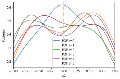
Here, pre-calibration performs comparable to adaptation, because the weights do not change so much over time. Note that one can also specify other scale functions, by passing AdaptiveAggregatedDistance(distances, scale_function), e.g. pyabc.distance.mean[/median/span].
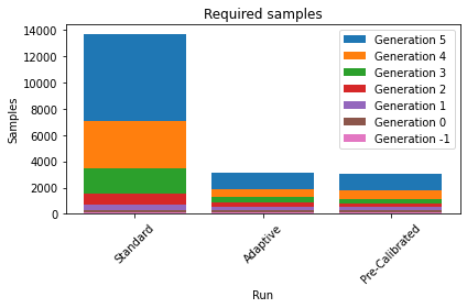
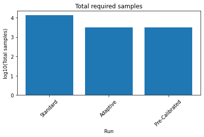
The following plots demonstrate that we not only have a much better posterior approximation after the same number of iterations in the second and third run compared to the first, but we achieve that actually with a much lower number of samples.
[6]:
histories = [history1, history2, history3]
labels = ['Standard', 'Adaptive', 'Pre-Calibrated']
pyabc.visualization.plot_sample_numbers(histories, labels, rotation=45)
pyabc.visualization.plot_total_sample_numbers(
histories, labels, yscale='log10', rotation=45
)
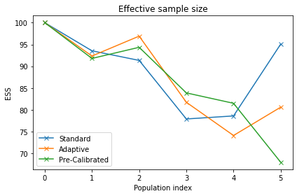
pyabc.visualization.plot_effective_sample_sizes(histories, labels)
[6]:
<AxesSubplot:title={'center':'Effective sample size'}, xlabel='Population index', ylabel='ESS'>