Early stopping of model simulations

This notebook can be downloaded here: Early Stopping.

For certain distance functions and certain models it is possible to calculate the distance on-the-fly while the model is running. This is e.g. possible if the distance is calculated as a cumulative sum and the model is a stochastic process. For example, Markov Jump Processes belong to this class. However, we want to keep things simple here and only demonstrate how to use the pyABC interface in such cases. So don’t expect a sophisticated (or even useful) model implementation here.

In this example we’ll use in particular the following classes for integrated simulation and accepting/rejecting a parameter:

• IntegratedModel

• ModelResult

Let’s start with the necessary imports:

# install if not done yet
!pip install pyabc --quiet

%matplotlib inline

import os
import tempfile

import matplotlib.pyplot as plt
import numpy as np
import pandas as pd

import pyabc
from pyabc import (
    ABCSMC,
    RV,
    Distribution,
    IntegratedModel,
    LocalTransition,
    MedianEpsilon,
    ModelResult,
    NoDistance,
)
from pyabc.sampler import SingleCoreSampler

pyabc.settings.set_figure_params('pyabc')  # for beautified plots

db_path = "sqlite:///" + os.path.join(tempfile.gettempdir(), "test.db")

We define here a (very) simple stochastic process, purely for demonstrative reasons. First, we fix the number of steps n_steps to 30.

n_steps = 30

We then define our process as follows:

\[x(t+1) = x(t) + s \xi,\]

in which \(\xi \sim U(0, 1)\) denotes a uniformly in \([0, 1]\) distributed random variable, and \(s\) is the step size, $s = $ step_size.

The function simulate implements this stochastic process:

def simulate(step_size):
    trajectory = np.zeros(n_steps)
    for t in range(1, n_steps):
        xi = np.random.uniform()
        trajectory[t] = trajectory[t - 1] + xi * step_size
    return trajectory

We take as distance function between two such generated trajectories the sum of the absolute values of the pointwise differences.

def distance(trajectory_1, trajectory_2):
    return np.absolute(trajectory_1 - trajectory_2).sum()

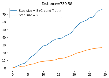
Let’s run the simulation and plot the trajectories to get a better idea of the so generated data. We set the ground truth step size gt_step_size to

gt_step_size = 5

This will be used to generate the data which will be subject to inference later on.

gt_trajectory = simulate(gt_step_size)
trajectoy_2 = simulate(2)

dist_1_2 = distance(gt_trajectory, trajectoy_2)

plt.plot(gt_trajectory, label=f"Step size = {gt_step_size} (Ground Truth)")
plt.plot(trajectoy_2, label="Step size = 2")
plt.legend()
plt.title(f"Distance={dist_1_2:.2f}");

As you might have noted already we could calculate the distance on the fly. After each step in the stochastic process, we could increment the cumulative sum. This will supposedly save time in the ABC-SMC run later on.

To implement this in pyABC we use the IntegratedModel.

Let’s start with the code first and explain it afterwards.

class MyStochasticProcess(IntegratedModel):
    def __init__(self, *args, **kwargs):
        super().__init__(*args, **kwargs)
        self.n_early_stopped = 0

    def integrated_simulate(self, pars, eps):
        cumsum = 0
        trajectory = np.zeros(n_steps)
        for t in range(1, n_steps):
            xi = np.random.uniform()
            next_val = trajectory[t - 1] + xi * pars["step_size"]
            cumsum += abs(next_val - gt_trajectory[t])
            trajectory[t] = next_val
            if cumsum > eps:
                self.n_early_stopped += 1
                return ModelResult(accepted=False)

        return ModelResult(
            accepted=True, distance=cumsum, sum_stat={"trajectory": trajectory}
        )

Our MyStochasticProcess class is a subclass of IntegratedModel <pyabc.model.IntegratedModel>.

The __init__ method is not really necessary. Here, we just want to keep track of how often early stopping has actually happened.

More interesting is the integrated_simulate method. This is where the real thing happens. As already said, we calculate the cumulative sum on the fly. In each simulation step, we update the cumulative sum. Note that gt_trajectory is actually a global variable here. If cumsum > eps at some step of the simulation, we return immediately, indicating that the parameter was not accepted by returning ModelResult(accepted=False). If the cumsum never passed eps, the parameter got accepted. In this case we return an accepted result together with the calculated distance and the trajectory. Note that, while it is mandatory to return the distance, returning the trajectory is optional. If it is returned, it is stored in the database.

We define a uniform prior over the interval \([0, 10]\) over the step size

prior = Distribution(step_size=RV("uniform", 0, 10))

and create and instance of our integrated model MyStochasticProcess

model = MyStochasticProcess()

We then configure the ABC-SMC run. As the distance function is calculated within MyStochasticProcess, we just pass None to the distance_function parameter. As sampler, we use the SingleCoreSampler here. We do so to correctly keep track of MyStochasticProcess.n_early_stopped. Otherwise, the counter gets incremented in subprocesses and we don’t see anything here. Of course, you could also use the MyStochasticProcess model in a multi-core or distributed setting.

Importantly, we pre-specify the initial acceptance threshold to a given value, here to 300. Otherwise, pyABC will try to automatically determine it by drawing samples from the prior and evaluating the distance function. However, we do not have a distance function here, so this approach would break down.

abc = ABCSMC(
    models=model,
    parameter_priors=prior,
    distance_function=NoDistance(),
    sampler=SingleCoreSampler(),
    population_size=30,
    transitions=LocalTransition(k_fraction=0.2),
    eps=MedianEpsilon(300, median_multiplier=0.7),
)

We then indicate that we want to start a new ABC-SMC run:

abc.new(db_path)

INFO:History:Start <ABCSMC id=1, start_time=2021-02-21 17:22:41.018237>

<pyabc.storage.history.History at 0x7f16e89e95e0>

We do not need to pass any data here. However, we could still pass additionally a dictionary {"trajectory": gt_trajectory} only for storage purposes to the new method. The data will however be ignored during the ABC-SMC run.

Then, let’s start the sampling

h = abc.run(minimum_epsilon=40, max_nr_populations=3)

INFO:ABC:t: 0, eps: 300.
INFO:ABC:Acceptance rate: 30 / 111 = 2.7027e-01, ESS=3.0000e+01.
INFO:ABC:t: 1, eps: 140.6687680285705.
INFO:ABC:Acceptance rate: 30 / 140 = 2.1429e-01, ESS=2.1150e+01.
INFO:ABC:t: 2, eps: 72.25140375797258.
INFO:ABC:Acceptance rate: 30 / 433 = 6.9284e-02, ESS=1.8744e+01.
INFO:pyabc.util:Stopping: maximum number of generations.
INFO:History:Done <ABCSMC id=1, duration=0:00:01.067589, end_time=2021-02-21 17:22:42.085826>

and check how often the early stopping was used:

model.n_early_stopped

594

Quite a lot actually.

Lastly we estimate KDEs of the different populations to inspect our results and plot everything (the vertical dashed line is the ground truth step size).

from pyabc.visualization import plot_kde_1d

fig, ax = plt.subplots()

for t in range(h.max_t + 1):
    particles = h.get_distribution(m=0, t=t)
    plot_kde_1d(
        *particles,
        "step_size",
        label=f"t={t}",
        ax=ax,
        xmin=0,
        xmax=10,
        numx=300,
    )
ax.axvline(gt_step_size, color="k", linestyle="dashed");

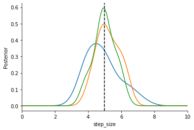
That’s it. You should be able to see how the distribution contracts around the true parameter.