Markov jump process: Reaction network

In the following, we fit stochastic chemical reaction kinetics with pyABC and show how to perform model selection between two competing models.

This notebook can be downloaded here: Markov Jump Process: Reaction Network.

We consider the two Markov jump process models \(m_1\) and \(m_2\) for conversion of (chemical) species \(X\) to species \(Y\):

\[\begin{split}m_1: X + Y \xrightarrow{k_1} 2Y\\ m_2: X \xrightarrow{k_2} Y.\end{split}\]

Each model is equipped with a single rate parameter \(k\). To simulate these models, we define a simple Gillespie simulator:

# install if not done yet
!pip install pyabc --quiet

import matplotlib.pyplot as plt
import numpy as np

from pyabc import ABCSMC, RV, Distribution
from pyabc.populationstrategy import AdaptivePopulationSize
from pyabc.visualization import plot_kde_1d


def h(x, pre, c):
    return (x**pre).prod(1) * c


def gillespie(x, c, pre, post, max_t):
    """
    Gillespie simulation

    Parameters
    ----------

    x: 1D array of size n_species
        The initial numbers.

    c: 1D array of size n_reactions
        The reaction rates.

    pre: array of size n_reactions x n_species
        What is to be consumed.

    post: array of size n_reactions x n_species
        What is to be produced

    max_t: int
        Timulate up to time max_t

    Returns
    -------
    t, X: 1d array, 2d array
        t: The time points.
        X: The history of the species.
           ``X.shape == (t.size, x.size)``

    """
    t = 0
    t_store = [t]
    x_store = [x.copy()]
    S = post - pre

    while t < max_t:
        h_vec = h(x, pre, c)
        h0 = h_vec.sum()
        if h0 == 0:
            break
        delta_t = np.random.exponential(1 / h0)
        # no reaction can occur anymore
        if not np.isfinite(delta_t):
            t_store.append(max_t)
            x_store.append(x)
            break
        reaction = np.random.choice(c.size, p=h_vec / h0)
        t = t + delta_t
        x = x + S[reaction]

        t_store.append(t)
        x_store.append(x)

    return np.array(t_store), np.array(x_store)

Next, we define the models in terms of ther initial molecule numbers \(x_0\), an array pre which determines what is to be consumed (the left hand side of the reaction equations) and an array post which determines what is to be produced (the right hand side of the reaction equations). Moreover, we define that the simulation time should not exceed MAX_T seconds.

Model 1 starts with initial concentrations \(X=40\) and \(Y=3\). The reaction \(X + Y \rightarrow 2Y\) is encoded in pre = [[1, 1]] and post = [[0, 2]].

MAX_T = 0.1


class Model1:
    __name__ = 'Model 1'
    x0 = np.array([40, 3])  # Initial molecule numbers
    pre = np.array([[1, 1]], dtype=int)
    post = np.array([[0, 2]])

    def __call__(self, par):
        t, X = gillespie(
            self.x0, np.array([float(par['rate'])]), self.pre, self.post, MAX_T
        )
        return {'t': t, 'X': X}

Model 2 inherits the initial concentration from model 1. The reaction \(X \rightarrow Y\) is incoded in pre = [[1, 0]] and post = [[0, 1]].

class Model2(Model1):
    __name__ = 'Model 2'
    pre = np.array([[1, 0]], dtype=int)
    post = np.array([[0, 1]])

We draw one stochastic simulation from model 1 (the “Observation”) and and one from model 2 (the “Competition”) and visualize both

%matplotlib inline

true_rate = 2.3
observations = [Model1()({'rate': true_rate}), Model2()({'rate': 30})]
fig, axes = plt.subplots(ncols=2)
fig.set_size_inches((12, 4))
for ax, title, obs in zip(axes, ['Observation', 'Competition'], observations):
    ax.step(obs['t'], obs['X'])
    ax.legend(['Species X', 'Species Y'])
    ax.set_xlabel('Time')
    ax.set_ylabel('Concentration')
    ax.set_title(title)

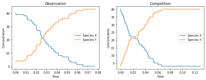
We observe that species \(X\) is converted into species \(Y\) in both cases. The difference of the concentrations over time can be quite subtle.

We define a distance function as \(L_1\) norm of two trajectories, evaluated at 20 time points:

\[\mathrm{distance}(X_1, X_2) = \frac{1}{N}\sum_{n=1}^{N} \left |X_1(t_n) -X_2(t_n) \right|, \quad t_n = \frac{n}{N}T, \quad N=20 \,.\]

Note that we only consider the concentration of species \(Y\) for distance calculation. And in code:

N_TEST_TIMES = 20

t_test_times = np.linspace(0, MAX_T, N_TEST_TIMES)


def distance(x, y):
    xt_ind = np.searchsorted(x['t'], t_test_times) - 1
    yt_ind = np.searchsorted(y['t'], t_test_times) - 1
    error = (
        np.absolute(x['X'][:, 1][xt_ind] - y['X'][:, 1][yt_ind]).sum()
        / t_test_times.size
    )
    return error

For ABC, we choose for both models a uniform prior over the interval \([0, 100]\) for their single rate parameters:

prior = Distribution(rate=RV('uniform', 0, 100))

We initialize the ABCSMC class passing the two models, their priors and the distance function.

abc = ABCSMC(
    [Model1(), Model2()],
    [prior, prior],
    distance,
    population_size=AdaptivePopulationSize(500),
)

ABC.Sampler INFO: Parallelize sampling on 2 processes.

We initialize a new ABC run, taking as observed data the one generated by model 1. The ABC run is to be stored in the sqlite database located at /tmp/mjp.db.

abc_id = abc.new('sqlite:////tmp/mjp.db', observations[0])

ABC.History INFO: Start <ABCSMC id=1, start_time=2026-04-14 16:41:32>

We start pyABC which automatically parallelizes across all available cores.

history = abc.run(minimum_epsilon=0.7, max_nr_populations=15)

ABC INFO: Calibration sample t = -1.
ABC INFO: t: 0, eps: 7.40000000e+00.
ABC INFO: Accepted: 500 / 1084 = 4.6125e-01, ESS: 5.0000e+02.
ABC.Adaptation INFO: Change nr particles 500 -> 2031
ABC INFO: t: 1, eps: 3.85000000e+00.
ABC INFO: Accepted: 2031 / 4946 = 4.1063e-01, ESS: 1.9546e+03.
ABC.Adaptation INFO: Change nr particles 2031 -> 1686
ABC INFO: t: 2, eps: 2.85000000e+00.
ABC INFO: Accepted: 1686 / 3559 = 4.7373e-01, ESS: 1.2246e+03.
ABC.Adaptation INFO: Change nr particles 1686 -> 1932
ABC INFO: t: 3, eps: 2.25000000e+00.
ABC INFO: Accepted: 1932 / 5371 = 3.5971e-01, ESS: 1.1036e+03.
ABC.Adaptation INFO: Change nr particles 1932 -> 2127
ABC INFO: t: 4, eps: 1.90000000e+00.
ABC INFO: Accepted: 2127 / 7932 = 2.6815e-01, ESS: 1.0230e+03.
ABC.Adaptation INFO: Change nr particles 2127 -> 2104
ABC INFO: t: 5, eps: 1.65000000e+00.
ABC INFO: Accepted: 2104 / 11612 = 1.8119e-01, ESS: 8.6365e+02.
ABC.Adaptation INFO: Change nr particles 2104 -> 2339
ABC INFO: t: 6, eps: 1.45000000e+00.
ABC INFO: Accepted: 2339 / 16359 = 1.4298e-01, ESS: 8.4619e+02.
ABC.Adaptation INFO: Change nr particles 2339 -> 2341
ABC INFO: t: 7, eps: 1.25000000e+00.
ABC INFO: Accepted: 2341 / 23758 = 9.8535e-02, ESS: 6.7510e+02.
ABC.Adaptation INFO: Change nr particles 2341 -> 2229
ABC INFO: t: 8, eps: 1.10000000e+00.
ABC INFO: Accepted: 2229 / 30511 = 7.3056e-02, ESS: 5.8426e+02.
ABC.Adaptation INFO: Change nr particles 2229 -> 2020
ABC INFO: t: 9, eps: 1.00000000e+00.
ABC INFO: Accepted: 2020 / 35085 = 5.7574e-02, ESS: 3.7508e+02.
ABC.Adaptation INFO: Change nr particles 2020 -> 2374
ABC INFO: t: 10, eps: 9.00000000e-01.
ABC INFO: Accepted: 2374 / 64790 = 3.6641e-02, ESS: 3.9307e+02.
ABC.Adaptation INFO: Change nr particles 2374 -> 2132
ABC INFO: t: 11, eps: 8.50000000e-01.
ABC INFO: Accepted: 2132 / 70114 = 3.0408e-02, ESS: 3.7636e+02.
ABC.Adaptation INFO: Change nr particles 2132 -> 2347
ABC INFO: t: 12, eps: 7.50000000e-01.
ABC INFO: Accepted: 2347 / 140734 = 1.6677e-02, ESS: 4.3589e+02.
ABC.Adaptation INFO: Change nr particles 2347 -> 2649
ABC INFO: t: 13, eps: 7.00000000e-01.
ABC INFO: Accepted: 2649 / 204518 = 1.2952e-02, ESS: 5.3251e+02.
ABC.Adaptation INFO: Change nr particles 2649 -> 2375
ABC INFO: Stop: Minimum epsilon.
ABC.History INFO: Done <ABCSMC id=1, duration=0:09:45.464765, end_time=2026-04-14 16:51:18>

We first inspect the model probabilities.

ax = history.get_model_probabilities().plot.bar()
ax.set_ylabel('Probability')
ax.set_xlabel('Generation')
ax.legend(
    [1, 2], title='Model', ncol=2, loc='lower center', bbox_to_anchor=(0.5, 1)
);

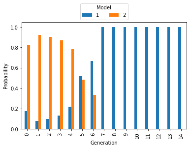
The mass at model 2 decreased, the mass at model 1 increased slowly. The correct model 1 is detected towards the later generations. We then inspect the distribution of the rate parameters:

fig, axes = plt.subplots(2)
fig.set_size_inches((6, 6))
axes = axes.flatten()
axes[0].axvline(true_rate, color='black', linestyle='dotted')
for m, ax in enumerate(axes):
    for t in range(0, history.n_populations, 2):
        df, w = history.get_distribution(m=m, t=t)
        if len(w) > 0:  # Particles in a model might die out
            plot_kde_1d(
                df,
                w,
                'rate',
                ax=ax,
                label=f't={t}',
                xmin=0,
                xmax=20 if m == 0 else 100,
                numx=200,
            )
    ax.set_title(f'Model {m+1}')
axes[0].legend(title='Generation', loc='upper left', bbox_to_anchor=(1, 1))

fig.tight_layout()

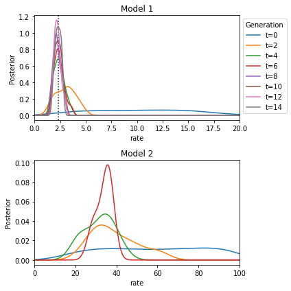
The true rate is closely approximated by the posterior over the rate of model 1. It is a little harder to interpret the posterior over model 2. Apparently a rate between 20 and 40 yields data most similar to the observed data.

Lastly, we visualize the evolution of the population sizes. The population sizes were automatically selected by pyABC and varied over the course of the generations. (We do not plot the size of th first generation, which was set to 500)

populations = history.get_all_populations()
ax = populations[populations.t >= 1].plot('t', 'particles', style='o-')
ax.set_xlabel('Generation');

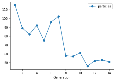
The initially chosen population size was adapted to the desired target accuracy. A larger population size was automatically selected by pyABC while both models were still alive. The population size decreased during the later populations thereby saving computational time.