PEtab application example

While the PEtab yaml2sbml notebook illustrates on a toy model the basics of the pyABC PEtab import, this notebook contains an application example based on real data.

# install if not done yet
!pip install pyabc --quiet

import os

import amici.petab_import
import numpy as np
import petab

import pyabc
from pyabc.petab import AmiciPetabImporter

We illustrate the usage of PEtab models using a model taken from the benchmark collection. The following cell clones the git repository.

!git clone --depth 1 https://github.com/LeonardSchmiester/Benchmark-Models.git \
    tmp/benchmark-models || (cd tmp/benchmark-models && git pull)

Cloning into 'tmp/benchmark-models'...
remote: Enumerating objects: 3511, done.
remote: Counting objects: 100% (3511/3511), done.
remote: Compressing objects: 100% (922/922), done.
remote: Total 3511 (delta 2695), reused 3170 (delta 2564), pack-reused 0
Receiving objects: 100% (3511/3511), 201.90 MiB | 20.18 MiB/s, done.
Resolving deltas: 100% (2695/2695), done.
Checking out files: 100% (3411/3411), done.

Now we can import a problem, here using the “Boehm_JProteomer2014” example, to AMICI and PEtab:

# read the petab problem from yaml
petab_problem = petab.Problem.from_yaml(
    "tmp/benchmark-models/hackathon_contributions_new_data_format/"
    "Boehm_JProteomeRes2014/Boehm_JProteomeRes2014.yaml"
)

# compile the petab problem to an AMICI ODE model
model = amici.petab_import.import_petab_problem(petab_problem)

# the solver to numerically solve the ODE
solver = model.getSolver()

# import everything to pyABC
importer = AmiciPetabImporter(petab_problem, model, solver)

# extract what we need from the importer
prior = importer.create_prior()
model = importer.create_model()
kernel = importer.create_kernel()

Once everything has been compiled and imported, we can simply call the model:

model(petab_problem.x_nominal_free_scaled)

{'llh': -138.22199570334107}

Now we can run an analysis using pyABC’s exact sequential sampler under the assumption of measurement noise. Note that the following cell takes, depending on the resources, minutes to hours to run through. Also, the resulting database is not provided here.

%%script false --no-raise-error
# Uncomment this line to run cell

# this takes some time

sampler = pyabc.MulticoreEvalParallelSampler(n_procs=20)

temperature = pyabc.Temperature()
acceptor = pyabc.StochasticAcceptor(
    pdf_norm_method = pyabc.ScaledPDFNorm())

abc = pyabc.ABCSMC(model, prior, kernel,
                   eps=temperature,
                   acceptor=acceptor,
                   sampler=sampler,
                   population_size=1000)
abc.new("sqlite:////tmp/petab_amici_boehm.db", {})
abc.run()

INFO:Sampler:Parallelizing the sampling on 20 cores.
INFO:History:Start <ABCSMC(id=1, start_time=2020-02-17 22:35:38.746712, end_time=None)>
INFO:ABC:Calibration sample before t=0.
INFO:ABC:t: 0, eps: 49386005.386943504.
INFO:ABC:Acceptance rate: 1000 / 3348 = 2.9869e-01, ESS=1.0000e+03.
INFO:ABC:t: 1, eps: 3707.524037573809.
INFO:ABC:Acceptance rate: 1000 / 3582 = 2.7917e-01, ESS=3.0162e+02.
INFO:ABC:t: 2, eps: 189.0069260595768.
INFO:ABC:Acceptance rate: 1000 / 3753 = 2.6645e-01, ESS=2.9065e+02.
INFO:ABC:t: 3, eps: 94.5034630297884.
INFO:ABC:Acceptance rate: 1000 / 6376 = 1.5684e-01, ESS=3.2931e+02.
INFO:ABC:t: 4, eps: 47.2517315148942.
INFO:ABC:Acceptance rate: 1000 / 16933 = 5.9056e-02, ESS=2.7417e+02.
INFO:ABC:t: 5, eps: 23.6258657574471.
INFO:ABC:Acceptance rate: 1000 / 6990 = 1.4306e-01, ESS=3.6511e+02.
INFO:ABC:t: 6, eps: 11.81293287872355.
INFO:ABC:Acceptance rate: 1000 / 50479 = 1.9810e-02, ESS=2.3205e+02.
INFO:ABC:t: 7, eps: 5.906466439361775.
INFO:ABC:Acceptance rate: 1000 / 141531 = 7.0656e-03, ESS=3.0510e+01.
INFO:ABC:t: 8, eps: 2.9532332196808877.
INFO:ABC:Acceptance rate: 1000 / 54532 = 1.8338e-02, ESS=2.7007e+01.
INFO:ABC:t: 9, eps: 1.4766166098404439.
INFO:ABC:Acceptance rate: 1000 / 21583 = 4.6333e-02, ESS=3.9807e+00.
INFO:ABC:t: 10, eps: 1.0.
INFO:ABC:Acceptance rate: 1000 / 12382 = 8.0762e-02, ESS=1.3817e+01.
INFO:ABC:Stopping: minimum epsilon.
INFO:History:Done <ABCSMC(id=1, start_time=2020-02-17 22:35:38.746712, end_time=2020-02-17 23:03:26.661874)>

<pyabc.storage.history.History at 0x7fa4da04f3a0>

Now we can use pyABC’s standard analysis and visualization routines to analyze the obtained posterior sample. In particular, we can extract boundaries and literature parameter values from the PEtab problem:

%%script false --no-raise-error
# Uncomment this line to run cell

h = pyabc.History("sqlite:///tmp/petab_amici_boehm.db", _id=1)
refval = {k: v for k,v in zip(petab_problem.x_free_ids, petab_problem.x_nominal_free_scaled)}
for i, par in enumerate(petab_problem.x_free_ids):
    pyabc.visualization.plot_kde_1d_highlevel(
        h, x=par,
        xmin=petab_problem.get_lb(scaled=True,fixed=False)[i],
        xmax=petab_problem.get_ub(scaled=True,fixed=False)[i],
        refval=refval, refval_color='k')

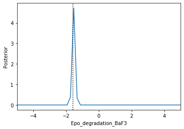
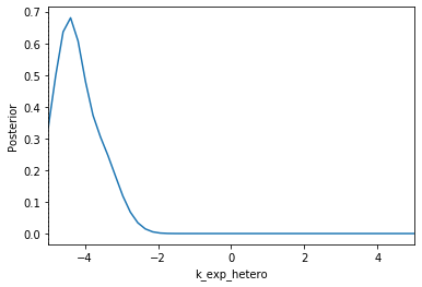
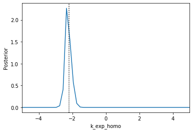
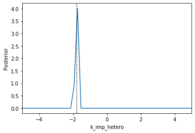
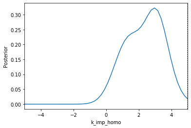
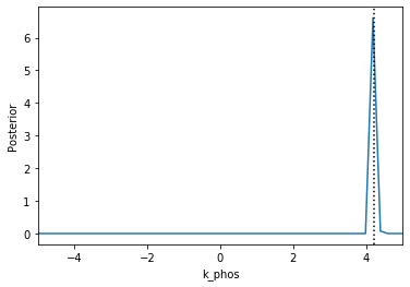
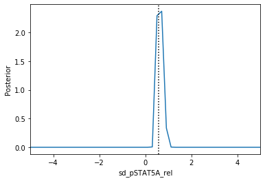
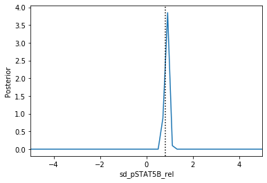
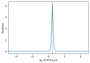
Apparently, in this case seven out of the nine parameters can be estimated with high confidence, while two other parameters can only be bounded.