Script based external simulators
In this notebook, we demonstrate the usage of the script based external simulators, summary statistics, and distance functions features.
These allow to use near-arbitrary programing languages and output for pyABC. The main concept is that all communication happens via the file system. This comes at the cost of a considerable overhead, making this feature not optimal for models with a low simulation time. For more expensive models, the overhead should be negligible.
This notebook is similar to the using_R notebook, but circumvents usage of the rpy2 package.
[ ]:
# install if not done yet
!pip install pyabc --quiet
[1]:
import os
from tempfile import gettempdir

import pyabc
import pyabc.external
from pyabc import ABCSMC, RV, Distribution
from pyabc.visualization import plot_kde_2d
Here, we define model, summary statistics and distance. Note that if possible, alternatively FileIdSumStat can be used to read in the summary statistics directly to python and then use a python based distance function.
[2]:
dir = 'model_r/'

model = pyabc.external.ExternalModel(
    executable='Rscript', file=f'{dir}/model.r'
)
sumstat = pyabc.external.ExternalSumStat(
    executable='Rscript', file=f'{dir}/sumstat.r'
)
distance = pyabc.external.ExternalDistance(
    executable='Rscript', file=f'{dir}/distance.r'
)

dummy_sumstat = (
    pyabc.external.create_sum_stat()
)  # can also use a real file here
[3]:
pars = {'meanX': 3, 'meanY': 4}
mf = model(pars)
print(mf)
sf = sumstat(mf)
print(sf)
distance(sf, dummy_sumstat)
{'loc': '/tmp/modelsim_0hz98kjx', 'returncode': 0}
{'loc': '/tmp/sumstat_ywmmq0pc', 'returncode': 0}
[3]:
4.834298
[4]:
prior = Distribution(meanX=RV('uniform', 0, 10), meanY=RV('uniform', 0, 10))
abc = ABCSMC(
    model, prior, distance, summary_statistics=sumstat, population_size=20
)

db = 'sqlite:///' + os.path.join(gettempdir(), 'test.db')
abc.new(db, dummy_sumstat)

history = abc.run(minimum_epsilon=0.9, max_nr_populations=4)
ABC.Sampler INFO: Parallelize sampling on 4 processes.
ABC.History INFO: Start <ABCSMC id=2, start_time=2021-11-18 15:45:50>
ABC INFO: Calibration sample t = -1.
ABC INFO: t: 0, eps: 3.34129400e+00.
ABC INFO: Accepted: 20 / 70 = 2.8571e-01, ESS: 2.0000e+01.
ABC INFO: t: 1, eps: 2.57219350e+00.
ABC INFO: Accepted: 20 / 45 = 4.4444e-01, ESS: 1.1949e+01.
ABC INFO: t: 2, eps: 2.12528659e+00.
ABC INFO: Accepted: 20 / 53 = 3.7736e-01, ESS: 1.8156e+01.
ABC INFO: t: 3, eps: 1.56643980e+00.
ABC INFO: Accepted: 20 / 65 = 3.0769e-01, ESS: 1.9740e+01.
ABC INFO: Stop: Maximum number of generations.
ABC.History INFO: Done <ABCSMC id=2, duration=0:01:20.956890, end_time=2021-11-18 15:47:11>
Note the significantly longer runtimes compared to using rpy2. This is because the simulation time of this model is very short, such that repeatedly accessing the file system creates a notable overhead. For more expensive models, this overhead however becomes less notable. Still, if applicable, more efficient ways of communication between model and simulator are preferable.
[5]:
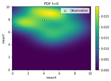
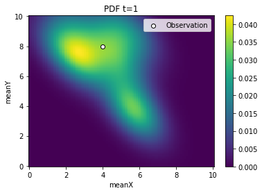
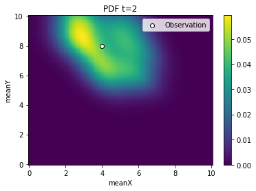
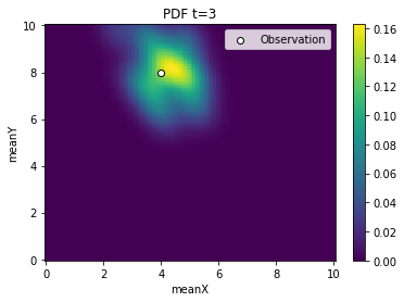
for t in range(history.n_populations):
    df, w = abc.history.get_distribution(0, t)
    ax = plot_kde_2d(
        df,
        w,
        'meanX',
        'meanY',
        xmin=0,
        xmax=10,
        ymin=0,
        ymax=10,
        numx=100,
        numy=100,
    )
    ax.scatter(
        [4], [8], edgecolor='black', facecolor='white', label='Observation'
    )
    ax.legend()
    ax.set_title(f'PDF t={t}')